

A differential analyzer is a mechanical, analog computer that can solve differential equations. Differential analyzers aren’t used anymore because even a cheap laptop can solve the same equations much faster—and can do it in the background while you stream the new season of Westworld on HBO. Before the invention of digital computers though, differential analyzers allowed mathematicians to make calculations that would not have been practical otherwise.
It is hard to see today how a computer made out of anything other than digital circuitry printed in silicon could work. A mechanical computer sounds like something out of a steampunk novel. But differential analyzers did work and even proved to be an essential tool in many lines of research. Most famously, differential analyzers were used by the US Army to calculate range tables for their artillery pieces. Even the largest gun is not going to be effective unless you have a range table to help you aim it, so differential analyzers arguably played an important role in helping the Allies win the Second World War.
To understand how differential analyzers could do all this, you will need to know what differential equations are. Forgotten what those are? That’s okay, because I had too.
Differential Equations
Differential equations are something you might first encounter in the final few weeks of a college-level Calculus I course. By that point in the semester, your underpaid adjunct professor will have taught you about limits, derivatives, and integrals; if you take those concepts and add an equals sign, you get a differential equation.
Differential equations describe rates of change in terms of some other variable (or perhaps multiple other variables). Whereas a familiar algebraic expression like \(y = 4x + 3\) specifies the relationship between some variable quantity \(y\) and some other variable quantity \(x\), a differential equation, which might look like \(\frac{dy}{dx} = x\), or even \(\frac{dy}{dx} = 2\), specifies the relationship between a rate of change and some other variable quantity. Basically, a differential equation is just a description of a rate of change in exact mathematical terms. The first of those last two differential equations is saying, “The variable \(y\) changes with respect to \(x\) at a rate defined exactly by \(x\),” and the second is saying, “No matter what \(x\) is, the variable \(y\) changes with respect to \(x\) at a rate of exactly 2.”
Differential equations are useful because in the real world it is often easier to describe how complex systems change from one instant to the next than it is to come up with an equation describing the system at all possible instants. Differential equations are widely used in physics and engineering for that reason. One famous differential equation is the heat equation, which describes how heat diffuses through an object over time. It would be hard to come up with a function that fully describes the distribution of heat throughout an object given only a time \(t\), but reasoning about how heat diffuses from one time to the next is less likely to turn your brain into soup—the hot bits near lots of cold bits will probably get colder, the cold bits near lots of hot bits will probably get hotter, etc. So the heat equation, though it is much more complicated than the examples in the last paragraph, is likewise just a description of rates of change. It describes how the temperature of any one point on the object will change over time given how its temperature differs from the points around it.
Let’s consider another example that I think will make all of this more concrete. If I am standing in a vacuum and throw a tennis ball straight up, will it come back down before I asphyxiate? This kind of question, posed less dramatically, is the kind of thing I was asked in high school physics class, and all I needed to solve it back then were some basic Newtonian equations of motion. But let’s pretend for a minute that I have forgotten those equations and all I can remember is that objects accelerate toward earth at a constant rate of \(g\), or about \(10 \;m/s^2\). How can differential equations help me solve this problem?
Well, we can express the one thing I remember about high school physics as a differential equation. The tennis ball, once it leaves my hand, will accelerate toward the earth at a rate of \(g\). This is the same as saying that the velocity of the ball will change (in the negative direction) over time at a rate of \(g\). We could even go one step further and say that the rate of change in the height of my ball above the ground (this is just its velocity) will change over time at a rate of negative \(g\). We can write this down as the following, where \(h\) represents height and \(t\) represents time:
\[\frac{d^2h}{dt^2} = -g\]This looks slightly different from the differential equations we have seen so far because this is what is known as a second-order differential equation. We are talking about the rate of change of a rate of change, which, as you might remember from your own calculus education, involves second derivatives. That’s why parts of the expression on the left look like they are being squared. But this equation is still just expressing the fact that the ball accelerates downward at a constant acceleration of \(g\).
From here, one option I have is to use the tools of calculus to solve the differential equation. With differential equations, this does not mean finding a single value or set of values that satisfy the relationship but instead finding a function or set of functions that do. Another way to think about this is that the differential equation is telling us that there is some function out there whose second derivative is the constant \(-g\); we want to find that function because it will give us the height of the ball at any given time. This differential equation happens to be an easy one to solve. By doing so, we can re-derive the basic equations of motion that I had forgotten and easily calculate how long it will take the ball to come back down.
But most of the time differential equations are hard to solve. Sometimes they are even impossible to solve. So another option I have, given that I paid more attention in my computer science classes that my calculus classes in college, is to take my differential equation and use it as the basis for a simulation. If I know the starting velocity and the acceleration of my tennis ball, then I can easily write a little for-loop, perhaps in Python, that iterates through my problem second by second and tells me what the velocity will be at any given second \(t\) after the initial time. Once I’ve done that, I could tweak my for-loop so that it also uses the calculated velocity to update the height of the ball on each iteration. Now I can run my Python simulation and figure out when the ball will come back down. My simulation won’t be perfectly accurate, but I can decrease the size of the time step if I need more accuracy. All I am trying to accomplish anyway is to figure out if the ball will come back down while I am still alive.
This is the numerical approach to solving a differential equation. It is how differential equations are solved in practice in most fields where they arise. Computers are indispensable here, because the accuracy of the simulation depends on us being able to take millions of small little steps through our problem. Doing this by hand would obviously be error-prone and take a long time.
So what if I were not just standing in a vacuum with a tennis ball but were standing in a vacuum with a tennis ball in, say, 1936? I still want to automate my computation, but Claude Shannon won’t even complete his master’s thesis for another year yet (the one in which he casually implements Boolean algebra using electronic circuits). Without digital computers, I’m afraid, we have to go analog.
The Differential Analyzer
The first differential analyzer was built between 1928 and 1931 at MIT by Vannevar Bush and Harold Hazen. Both men were engineers. The machine was created to tackle practical problems in applied mathematics and physics. It was supposed to address what Bush described, in a 1931 paper about the machine, as the contemporary problem of mathematicians who are “continually being hampered by the complexity rather than the profundity of the equations they employ.”
A differential analyzer is a complicated arrangement of rods, gears, and spinning discs that can solve differential equations of up to the sixth order. It is like a digital computer in this way, which is also a complicated arrangement of simple parts that somehow adds up to a machine that can do amazing things. But whereas the circuitry of a digital computer implements Boolean logic that is then used to simulate arbitrary problems, the rods, gears, and spinning discs directly simulate the differential equation problem. This is what makes a differential analyzer an analog computer—it is a direct mechanical analogy for the real problem.
How on earth do gears and spinning discs do calculus? This is actually the easiest part of the machine to explain. The most important components in a differential analyzer are the six mechanical integrators, one for each order in a sixth-order differential equation. A mechanical integrator is a relatively simple device that can integrate a single input function; mechanical integrators go back to the 19th century. We will want to understand how they work, but, as an aside here, Bush’s big accomplishment was not inventing the mechanical integrator but rather figuring out a practical way to chain integrators together to solve higher-order differential equations.
A mechanical integrator consists of one large spinning disc and one much smaller spinning wheel. The disc is laid flat parallel to the ground like the turntable of a record player. It is driven by a motor and rotates at a constant speed. The small wheel is suspended above the disc so that it rests on the surface of the disc ever so slightly—with enough pressure that the disc drives the wheel but not enough that the wheel cannot freely slide sideways over the surface of the disc. So as the disc turns, the wheel turns too.
The speed at which the wheel turns will depend on how far from the center of the disc the wheel is positioned. The inner parts of the disc, of course, are rotating more slowly than the outer parts. The wheel stays fixed where it is, but the disc is mounted on a carriage that can be moved back and forth in one direction, which repositions the wheel relative to the center of the disc. Now this is the key to how the integrator works: The position of the disc carriage is driven by the input function to the integrator. The output from the integrator is determined by the rotation of the small wheel. So your input function drives the rate of change of your output function and you have just transformed the derivative of some function into the function itself—which is what we call integration!
If that explanation does nothing for you, seeing a mechanical integrator in action really helps. The principle is surprisingly simple and there is no way to watch the device operate without grasping how it works. So I have created a visualization of a running mechanical integrator that I encourage you to take a look at. The visualization shows the integration of some function \(f(x)\) into its antiderivative \(F(x)\) while various things spin and move. It’s pretty exciting.
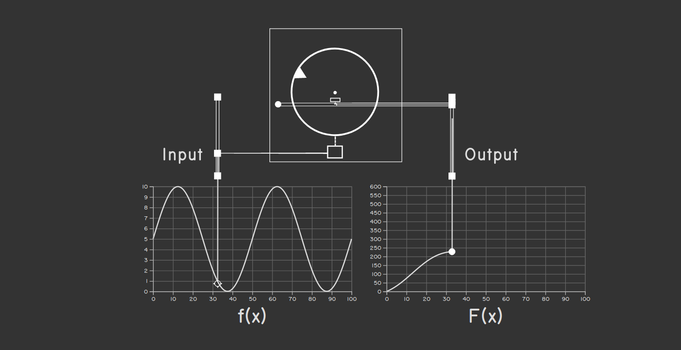 A nice screenshot of my visualization, but you should check out the real
thing!
A nice screenshot of my visualization, but you should check out the real
thing!
So we have a component that can do integration for us, but that alone is not enough to solve a differential equation. To explain the full process to you, I’m going to use an example that Bush offers himself in his 1931 paper, which also happens to be essentially the same example we contemplated in our earlier discussion of differential equations. (This was a happy accident!) Bush introduces the following differential equation to represent the motion of a falling body:
\[\frac{d^2x}{dt^2} = -k\,\frac{dx}{dt} - g\]This is the same equation we used to model the motion of our tennis ball, only Bush has used \(x\) in place of \(h\) and has added another term that accounts for how air resistance will decelerate the ball. This new term describes the effect of air resistance on the ball in the simplest possible way: The air will slow the ball’s velocity at a rate that is proportional to its velocity (the \(k\) here is some proportionality constant whose value we don’t really care about). So as the ball moves faster, the force of air resistance will be stronger, further decelerating the ball.
To configure a differential analyzer to solve this differential equation, we have to start with what Bush calls the “input table.” The input table is just a piece of graphing paper mounted on a carriage. If we were trying to solve a more complicated equation, the operator of the machine would first plot our input function on the graphing paper and then, once the machine starts running, trace out the function using a pointer connected to the rest of the machine. In this case, though, our input is just the constant \(g\), so we only have to move the pointer to the right value and then leave it there.
What about the other variables \(x\) and \(t\)? The \(x\) variable is our output as it represents the height of the ball. It will be plotted on graphing paper placed on the output table, which is similar to the input table only the pointer is a pen and is driven by the machine. The \(t\) variable should do nothing more than advance at a steady rate. (In our Python simulation of the tennis ball problem as posed earlier, we just incremented \(t\) in a loop.) So the \(t\) variable comes from the differential analyzer’s motor, which kicks off the whole process by rotating the rod connected to it at a constant speed.
Bush has a helpful diagram documenting all of this that I will show you in a second, but first we need to make one more tweak to our differential equation that will make the diagram easier to understand. We can integrate both sides of our equation once, yielding the following:
\[\frac{dx}{dt} = - \int \left(k\,\frac{dx}{dt} + g\right)\,dt\]The terms in this equation map better to values represented by the rotation of various parts of the machine while it runs. Okay, here’s that diagram:
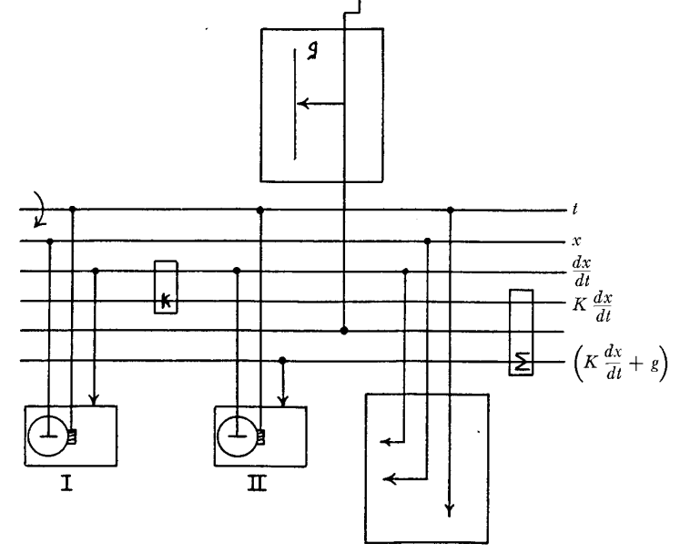 The differential analyzer configured to solve the problem of a falling body in
one dimension.
The differential analyzer configured to solve the problem of a falling body in
one dimension.
The input table is at the top of the diagram. The output table is at the bottom-right. The output table here is set up to graph both \(x\) and \(\frac{dx}{dt}\), i.e. height and velocity. The integrators appear at the bottom-left; since this is a second-order differential equation, we need two. The motor drives the very top rod labeled \(t\). (Interestingly, Bush referred to these horizontal rods as “buses.”)
That leaves two components unexplained. The box with the little \(k\) in it is a multiplier respresnting our proportionality constant \(k\). It takes the rotation of the rod labeled \(\frac{dx}{dt}\) and scales it up or down using a gear ratio. The box with the \(\sum\) symbol is an adder. It uses a clever arrangement of gears to add the rotations of two rods together to drive a third rod. We need it since our equation involves the sum of two terms. These extra components available in the differential analyzer ensure that the machine can flexibly simulate equations with all kinds of terms and coefficients.
I find it helpful to reason in ultra-slow motion about the cascade of cause and effect that plays out as soon as the motor starts running. The motor immediately begins to rotate the rod labeled \(t\) at a constant speed. Thus, we have our notion of time. This rod does three things, illustrated by the three vertical rods connected to it: it drives the rotation of the discs in both integrators and also advances the carriage of the output table so that the output pen begins to draw.
Now if the integrators were set up so that their wheels are centered, then the rotation of rod \(t\) would cause no other rods to rotate. The integrator discs would spin but the wheels, centered as they are, would not be driven. The output chart would just show a flat line. This happens because we have not accounted for the initial conditions of the problem. In our earlier Python simulation, we needed to know the initial velocity of the ball, which we would have represented there as a constant variable or as a parameter of our Python function. Here, we account for the initial velocity and acceleration by displacing the integrator discs by the appropriate amount before the machine begins to run.
Once we’ve done that, the rotation of rod \(t\) propagates through the whole system. Physically, a lot of things start rotating at the same time, but we can think of the rotation going first to integrator II, which combines it with the acceleration expression calculated based on \(g\) and then integrates it to get the result \(\frac{dx}{dt}\). This represents the velocity of the ball. The velocity is in turn used as input to integrator I, whose disc is displaced so that the output wheel rotates at the rate \(\frac{dx}{dt}\). The output from integrator I is our final output \(x\), which gets routed directly to the output table.
One confusing thing I’ve glossed over is that there is a cycle in the machine: Integrator II takes as an input the rotation of the rod labeled \((k\,\frac{dx}{dt} + g)\), but that rod’s rotation is determined in part by the output from integrator II itself. This might make you feel queasy, but there is no physical issue here—everything is rotating at once. If anything, we should not be surprised to see cycles like this, since differential equations often describe rates of change in a function as a function of the function itself. (In this example, the acceleration, which is the rate of change of velocity, depends on the velocity.)
With everything correctly configured, the output we get is a nice graph, charting both the position and velocity of our ball over time. This graph is on paper. To our modern digital sensibilities, that might seem absurd. What can you do with a paper graph? While it’s true that the differential analyzer is not so magical that it can write out a neat mathematical expression for the solution to our problem, it’s worth remembering that neat solutions to many differential equations are not possible anyway. The paper graph that the machine does write out contains exactly the same information that could be output by our earlier Python simulation of a falling ball: where the ball is at any given time. It can be used to answer any practical question you might have about the problem.
The differential analyzer is a preposterously cool machine. It is complicated, but it fundamentally involves nothing more than rotating rods and gears. You don’t have to be an electrical engineer or know how to fabricate a microchip to understand all the physical processes involved. And yet the machine does calculus! It solves differential equations that you never could on your own. The differential analyzer demonstrates that the key material required for the construction of a useful computing machine is not silicon but human ingenuity.
Murdering People
Human ingenuity can serve purposes both good and bad. As I have mentioned, the highest-profile use of differential analyzers historically was to calculate artillery range tables for the US Army. To the extent that the Second World War was the “Good Fight,” this was probably for the best. But there is also no getting past the fact that differential analyzers helped to make very large guns better at killing lots of people. And kill lots of people they did—if Wikipedia is to be believed, more soldiers were killed by artillery than small arms fire during the Second World War.
I will get back to the moralizing in a minute, but just a quick detour here to explain why calculating range tables was hard and how differential analyzers helped, because it’s nice to see how differential analyzers were applied to a real problem. A range table tells the artilleryman operating a gun how high to elevate the barrel to reach a certain range. One way to produce a range table might be just to fire that particular kind of gun at different angles of elevation many times and record the results. This was done at proving grounds like the Aberdeen Proving Ground in Maryland. But producing range tables solely through empirical observation like this is expensive and time-consuming. There is also no way to account for other factors like the weather or for different weights of shell without combinatorially increasing the necessary number of firings to something unmanageable. So using a mathematical theory that can fill in a complete range table based on a smaller number of observed firings is a better approach.
I don’t want to get too deep into how these mathematical theories work, because the math is complicated and I don’t really understand it. But as you might imagine, the physics that governs the motion of an artillery shell in flight is not that different from the physics that governs the motion of a tennis ball thrown upward. The need for accuracy means that the differential equations employed have to depart from the idealized forms we’ve been using and quickly get gnarly. Even the earliest attempts to formulate a rigorous ballistic theory involve equations that account for, among other factors, the weight, diameter, and shape of the projectile, the prevailing wind, the altitude, the atmospheric density, and the rotation of the earth1.
So the equations are complicated, but they are still differential equations that a differential analyzer can solve numerically in the way that we have already seen. Differential analyzers were put to work solving ballistics equations at the Aberdeen Proving Ground in 1935, where they dramatically sped up the process of calculating range tables.2 Nevertheless, during the Second World War, the demand for range tables grew so quickly that the US Army could not calculate them fast enough to accompany all the weaponry being shipped to Europe. This eventually led the Army to fund the ENIAC project at the University of Pennsylvania, which, depending on your definitions, produced the world’s first digital computer. ENIAC could, through rewiring, run any program, but it was constructed primarily to perform range table calculations many times faster than could be done with a differential analyzer.
Given that the range table problem drove much of the early history of computing even apart from the differential analyzer, perhaps it’s unfair to single out the differential analyzer for moral hand-wringing. The differential analyzer isn’t uniquely compromised by its military applications—the entire field of computing, during the Second World War and well afterward, advanced because of the endless funding being thrown at it by the United States military.
Anyway, I think the more interesting legacy of the differential analyzer is what it teaches us about the nature of computing. I am surprised that the differential analyzer can accomplish as much as it can; my guess is that you are too. It is easy to fall into the trap of thinking of computing as the realm of what can be realized with very fast digital circuits. In truth, computing is a more abstract process than that, and electronic, digital circuits are just what we typically use to get it done. In his paper about the differential analyzer, Vannevar Bush suggests that his invention is just a small contribution to “the far-reaching project of utilizing complex mechanical interrelationships as substitutes for intricate processes of reasoning.” That puts it nicely.
If you enjoyed this post, more like it come out every four weeks! Follow @TwoBitHistory on Twitter or subscribe to the RSS feed to make sure you know when a new post is out.
Previously on TwoBitHistory…
Do you worry that your children are "BBS-ing"? Do you have a neighbor who talks too much about his "door games"?
— TwoBitHistory (@TwoBitHistory) February 2, 2020
In this VICE News special report, we take you into the seedy underworld of bulletin board systems:https://t.co/hBrKGU2rfB
-
Alan Gluchoff. “Artillerymen and Mathematicians: Forest Ray Moulton and Changes in American Exterior Ballistics, 1885-1934.” Historia Mathematica, vol. 38, no. 4, 2011, pp. 506–547., https://www.sciencedirect.com/science/article/pii/S0315086011000279. ↩
-
Karl Kempf. “Electronic Computers within the Ordnance Corps,” 1961, accessed April 6, 2020, https://ftp.arl.army.mil/~mike/comphist/61ordnance/index.html. ↩